Chi-square
The chi-square analysis is a useful and relatively flexible tool for determining if categorical variables are related.
There are various ways to run chi-square analyses in Stata. In addition to the built-in function encompassed by tabulate there is a fairly nice user-created package (findit tab chi cox and select the first package found - this package is used with the command chitesti). Which one you use depends on what type of chi-square you want to perform (single variable versus multiple variables).
Chi-square for Goodness of Fit
To run a chi-square for goodness of fit, you are going to need the package described above. This package does not require that you use a dataset. Instead, you simply tell STATA both the observed and the expected frequencies and let it take care of the math. The syntax for the command is as follows chitesti #observed1 #oberved2 #observedN \ #expected1 #expected2 #expectedN where N implies the command can go on as long as it needs to. Alternatively, you can use chitest [variable for observed] [variable for expected] which will just pull the observed and expected data from columns rather than user input. In either case, if no expected values are specified Stata assumes you expect an equal distribution.
For example, perhaps I have hypothesized that Reed students make different pet choices than do Portlanders. I spent a complete day in Commons stopping people as they leave, making sure they're not prospies, staff or faculty, and asking what kind of pet they have. Then, because I don't want sample bias, I spend another day outside of the Library and a third outside the Sports Center. In the end, I have three hundred tallymarks divided into three categories: big mammals (dogs, cats): 106, small creatures (birds, rabbits, rats, etc):55, fish/none:137, exotics (difficult sealife, snakes, etc.): 2. I compare this data to some data from the (made up for this example) Portland Pet People Project which says that 65% of Portlanders own a dog or a cat, 15% own what I classified as a small creature, 19% own fish or no pet, and 1% own something more exotic. Some quick math informs me that in my sample of 300, that makes my expected values big mammals: 195, small mammals: 45, none/fish: 57 and exotics: 3. Therefore, the Stata command is as follows: chitesti 106 55 137 2 \ 195 45 57 3 and yields the following output:
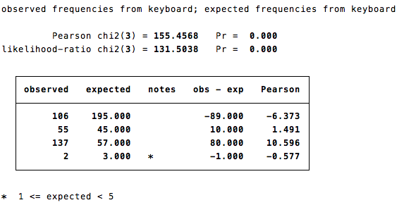
We are given the raw chi-square value and corresponding p-value (here, p<.001), as well as a calculated likelihood-ratio chi value.
Then we are given a table of the actual observed and expected frequencies for each category. This is a good way to check that you did not enter any values incorrectly. The note at the end of the output corresponds to the asterisk, which indicates that one cell was expected to have less than 5 observations (which could pose problems in analyses).
For more information on this package, once it is installed, you can use the command help chitesti
Chi-square for Independence
To run a chi-square for independence, you can use either the package explained above or the tabulate command (abbreviated to tab for the duration of this explanation). In either case, this command will require a loaded dataset. The tab command takes arguments as follows tab [categorical var] [categorical var2], chi2 and will only compute a chi-square if the chi2 option is specified. It is okay to have more than two variables, but may make it harder to come to meaningful conclusions as the table gets more complicated. The tabchi command is similar but will take at most two variables (see help tabchi for more on this option).
For this example, pretend I am studying movie genre preference by gender using ticket sales. If you already have this data in a long format (one person per line) then the command is simply tab gender genre, chi2 which (using my made-up data) produces the following output:
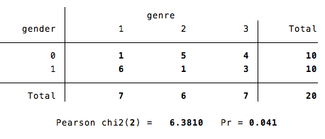
The output is simple: we are given a table of observed frequences, followed by the chi-square value and p-value.
If you do not already have a dataset, it is quick and easy to set one up (wide form) specifically for the purposes of conducting the analysis. Basically, you need one column for each variable and a final column for the count. When you set the data up like this, each row is a different combination of the variables of interest. So continuing the example above, the data would look as follows
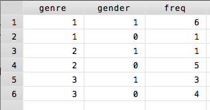
The command itself is nearly the same as before, but modified to tell Stata that there is a frequency variable by adding [freq=[frequency variable]] with the brackets. Therefore, the command in total reads tab gender genre [freq=freq], chi2 and displays the exact same output as the original command run on the data in long form.