Spring 2010
Econometric Project #5
Instrumental Variables and System Estimation
Due 6am, Tuesday, April 6
This project contains three exercises. The first two are quite short extensions of work you have done before. The last is new and somewhat longer.
Project Teams
Project teams for this assignment are below. You should make contact with your partner as soon as possible to arrange a work schedule.
| Skye Aaron | Li Zha |
| Raphael Deem | Thomas Verghese |
| Andrew Dubay | Erik Swanson |
| Tian Jiang | Justin Stewart |
| Robert Kahn | Nina Showell |
| David Krueger | Trey Sands |
| Ethan Knudson | Cori Savaiano |
| Tyrone Lee | Suraj Pant |
| Luis López | Kelsey Lucas |
Exercise 1: Airfares redux
In the final exercise of Project #3, you all concluded that the variable measuring passengers per day was probably endogenous to the determination of airfares. We now explore that using instrumental variables. Once again, we use the airfare.dta dataset.
a. Estimating a demand or supply function
We may think of airfares and number of passengers as being jointly determined by the demand and supply for air travel on that route in that year. In addition to fare and passengers, we have two route-specific variables: distance and market concentration. We also have the identities of the cities involved in the route and, as you know, can construct dummy variables for them. Which of these variables is likely to affect the demand curve, which the supply curve, and which would affect both? Based on your assumptions, assess the identification status of each equation and estimate any equation(s) that is (are) identified using two-stage least squares.
You may include time dummies or city dummies if you think it's appropriate, or use a fixed-effects or random-effects estimator if you think that's the right specification. (Combining instrumental variables with panel data estimators can be done with xtivreg in Stata.)
Are your results reasonable? If possible, test your assumptions about the relevance and/or exogeneity of your instruments.
b. Improving the specification
What additional variables would you like to have in order to improve the estimates of the demand and supply curves in part a? Which ones might be feasible to collect from data sources to which you have access? Try to find a sources for these variables, then design and describe in detail a plan to perform your improved estimates. (You don't have to actually carry out the plan.)
Exercise 2: Fertility redux
In Project #4, you worked with a dataset on fertility. In particular, you explored how the decision to have additional children was affected by the sex of the first two children.
For this exercise, you are to continue this research by examining how the number of children affects women's labor supply, using your work from Project #4 as a basis. Working women are probably less likely to have additional children, so the morekids variable is likely endogenous in the labor-supply equation.
Stock and Watson's Empirical Exercise E12.2 suggests an approach to looking at the effect of number of children on women's labor supply. Perform an analysis of this question using the fertility dataset. You should conduct all of the procedures suggested in Exercise E12.2, but you may want to explore the problem more completely.
Write up your results as an essay rather than as individual answers to the parts of E12.2.
Exercise 3: Estimating inter-related cost and input-demand functions
This exercise is derived from exercises in Berndt's Chapter 9. You may wish to read his Section 9.2 for more detail.
After the sharp rise in oil prices in the 1970s, economists turned their attention to trying to estimate the elasticity of the demand for oil and other energy goods. Because much of U.S. energy use is in the production of other goods and services, a major focus of that analysis was on the demand for energy as an input to production. The analysis of the demand for energy as a factor of production was a convenient application of some advances in micro-econometrics that had occurred a few years earlier.
As we discussed earlier in the semester (in our discussion of costs when we considered economies of scale), the technology of production can be equivalently characterized either by a production function (relating output quantity to input quantities) or by a cost function (relating total cost to input prices and output quantity) that is uniquely related to (dual to) the production function. Given the cost function, Shephard's Lemma tells us that the demand function for each input is the partial derivative of the cost function with respect to that input's price.
Estimation of these cost and input-demand functions required the development of new "flexible" functional forms that would make the functions linear in parameters, but also retain the essential properties of cost functions---in particular, that the cost function must be homogeneous of degree one in all prices so that a doubling of all prices leads to a doubling of costs. Among the flexible functional forms that emerged in the early 1970s, the two most popular were the transcendental logarithmic (translog) function, in which the log of costs is a quadratic function of the logs of the input prices (and the quantity of output) and the generalized Leontief (GL) function in which average cost is quadratic in the square roots of the input prices. The detailed description of the GL function and the input-demand functions derived from it are in this supporting document.
The dataset klem.dta contains data from Ernst Berndt's own research on aggregate U.S. manufacturing input quantities and prices for the 1947-71 period---much the same data he used to estimate energy demand at the onset of the energy crisis. Although these are time-series data, we are going to ignore any problems of serial correlation or non-stationarity in estimating these equations and treat the observations as though they are IID.
a. Examination of the GL function
Verify that the GL function has the property of linear homogeneity and that the input-demand functions are homogeneous of degree zero in prices. In other words, a doubling of all price variables will exactly double costs and will leave all input demands unchanged. Does the GL function as given in this project allow for non-constant returns to scale? How might you change it if you wanted to examine returns to scale? How would this change the input-demand functions? Could you still estimate them in the same form?
b. OLS estimation of input demands
To provide a benchmark, estimate each of the four input-demand equations separately by OLS. How well do the equations fit? How statistically significant are the coefficients? Do the symmetry restrictions dij = dji appear to hold for your estimates?
One key question of interest at the time was whether the cross-price elasticity of demand between energy and capital was positive or negative. The effect of energy (capital) price on capital (energy) demand is measured by dKE. A positive value would indicate a degree of substitutability between capital and energy, so that the demand for capital increases with an increase in energy prices. A negative value would indicate complementarity between capital and energy. What do your results suggest? Do you get the same result from the capital equation as from the energy equation?
c. Seemingly unrelated regressions
Now estimate the four equations together as a system of equations using the technique of iterated seemingly unrelated regressions, initially not imposing the symmetry restrictions that dij = dji. How different are the results? Does it appear that the added efficiency gained by accounting for the cross-equation correlation of the error terms has substantially altered your estimates?
Compare the results of your OLS and SUR estimation to those reported by Berndt in Table 9.1 (reproduced below). Any differences?
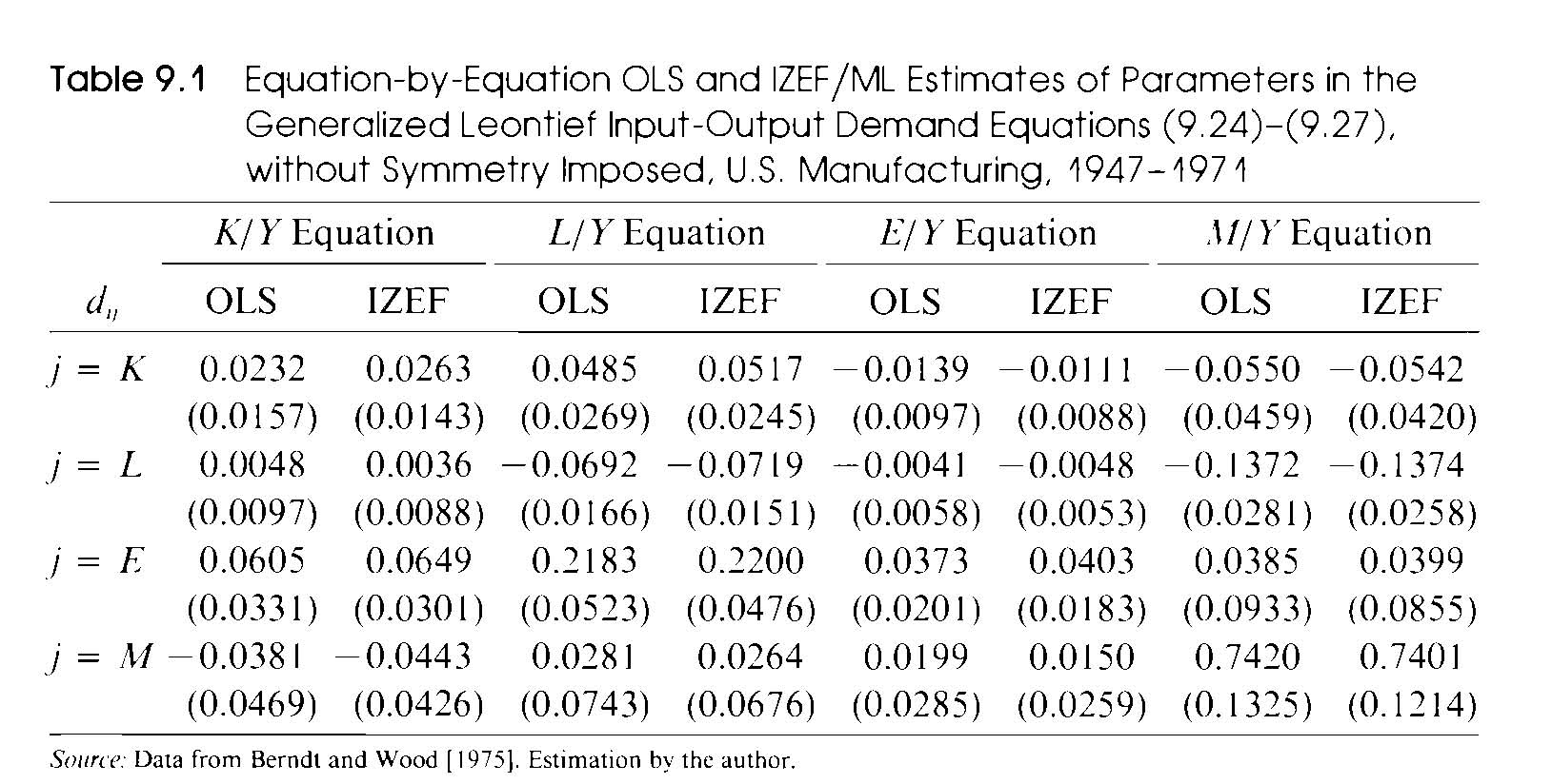
Does this change your conclusions about capital/energy substitutability?
d. Imposing and testing the symmetry restrictions
Now test the symmetry restrictions using the SUR estimates. What would if mean to reject the symmetry restrictions? Are you able to reject the symmetry restrictions on the model?
Run the SUR regressions imposing the symmetry restrictions. How does imposing the restrictions affect the qualitative conclusions about the effects of input prices and quantities, both in general and for the special case of capital/energy substitutability?
e. Dealing with endogenous input prices
With aggregate data of this kind, it is difficult to argue that input prices are unaffected by shocks to the overall demand by U.S. manufacturers for the inputs. Berndt provides a set of 10 instruments that are assumed to be exogenous. They are called z1 through z10 in the dataset and are defined on page 487 of his text.
Use these instruments to re-run your regressions for part (b) above using two-stage least squares. Are your results qualitatively different? Does controlling for endogeneity seem to affect the estimates much? Are your instruments relevant? Do they seem to be exogenous?
Now repeat parts (c) and (d) using three-stage least squares. How are your results affected?
f. Conclusions
Summarize your conclusions from estimation of input-demand functions for U.S. manufacturing.