tidynlm and Cholera
Jackson M Luckey
library(tidyverse)
library(tidynlm)
What is tidynlm?
tidynlm provides easy access to the National Library of Medicine (NLM) API from within R. The package allows the user to create a dataframe of NLM documents matching a particular search query using the function searchnlm. The resulting dataframe contains information on attributes such as authorship and date and place of publication. The documents themselves can be accessed with the urls in the url column of the resulting dataframe. I wrote the package because I could not find another convenient way to query the NLM database.
Installation
You can install tidynlm from GitHub with:
# install.packages("devtools")
devtools::install_github("https://github.com/Reed-Statistics/book_trackR")
How tidynlm Works
APIs, or Application Programmable Interface, is a specification for how software components communicate with each other. In this case, the API provides access to the National Library of Medicine’s database of medical documents. tidynlm is an API wrapper, meaning that it writes and executes API queries on the user’s behalf. In order to do so, searchnlm–the main function of tidynlm–manipulates its inputs (e.g. term, field) into a URL. It then loads the XML document that the URL provides access to, and parses it into a dataframe. More information about the National Library of Medicine API is available here.
searchnlm starts by reformatting the term input to match the NLM’s API. It replaces spaces with “+”s to represent ANDs, and collapses the vector into a single string separated by “+OR+”s to represent ORs. If field is included, it prefixes the term in “dc:field:”. Finally, the whole term is added to “https://wsearch.nlm.nih.gov/ws/query?db=digitalCollection&term=”, which is the base URL for the NLM API. By base URL, I mean the part of the URL that is the same for all API requests.
searchnlm then queries the URL with the read_xml function from the xml2 package. This function parses the raw XML associated with the URL. XML, or Extensible Markup Language, “is a simple text-based format for representing structured information: documents, data… and much more”. You can read more about XML here. After parsing the XML, searchnlm uses functions from xml2, dplyr, and tidyr to restructure the data as a dataframe. If output is set to “wide”, then each row in the final dataframe will be a specific document in the NLM database. Otherwise, each row will be a field in the XML that refers to a specific document. Finally, if collapse_to_first is set to TRUE, duplicated fields will be dropped. This makes working with the dataframe much easier, but risks losing crucial information. Otherwise, duplicated fields will result in a list-column–that is, columns that may contain multiple elements.
You can find out more in R after installing and loading tidynlm with the following commands:
?tidynlm
?searchnlm
You can read more about the National Library of Medicine API here.
Cholera
What is Cholera
Cholera is a “is an acute diarrhoeal infection caused by ingestion of food or water contaminated with the bacterium Vibrio cholerae”. Modern public health partially emerged from combating Cholera, which is often spread through contaminated water supplies. The disease is easily controlled with sanitation and hygiene, but without it, the disease causes deadly cyclical epidemics. It spread worldwide during the 19th century, and is a useful indicator of inequality and a lack of development. You can find out more about Cholera from the World Health Organization and the Center for Disease Control.
History of Cholera Publications
cholera <- searchnlm(term = "cholera", retmax = 10000, output = "wide", collapse_to_first = TRUE)We will start by graphing the number of documents pertaining to Cholera in the National Library of Medicine by year. To do so, we will first query the NLM database using searchnlm with output set to “wide” and collapse_to_first set to TRUE. This ensures that each row is a document, and that none of the variables are list-columns, which makes working with the dataset much easier. We will then aggregate the resulting dataframe by year using group_by and count and plot it with ggplot. As can be seen below, the National Library of Medicine’s documents on Cholera primarily date to the later half of the 19th century. This makes sense, given that Cholera spread worldwide in the 19th century, and was controlled in most wealthy countries by the early 1900s.
 cholera %>%
  mutate(date = as.numeric(date)) %>%
  group_by(date) %>%
  count() %>%
  ungroup() %>%
  ggplot(aes(x = date, y = n)) +
  geom_point() +
  xlim(1770, 2020) +
  theme_classic() +
  labs(x = "Year",
       y = "Number of Documents",
       title = "Number of Documents Involving Cholera by Year",
       subtitle = "National Library of Medicine")
## Warning: Removed 8 rows containing missing values (geom_point).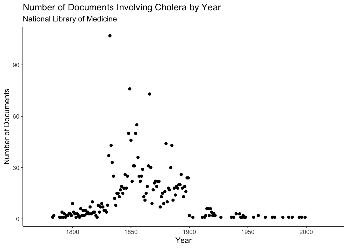
Now let’s look at the language composition of the documents in the National Library of Medicine. We will be working with the same cholera dataset we produced earlier. As you can see below, the vast majority of the documents are written in English. This is unsurprising as the National Library of Medicine is administered by a predominantly English-speaking country (the United States). Interestingly, Portuguese is the second most common language. I would have guessed that it would be French, German, or Latin, given their extensive use in medicine and science in the 19th century.
Cholera Publications by Language
cholera %>%
  ggplot(aes(x = fct_infreq(language))) +
  geom_bar() +
  theme_classic() +
  coord_flip() +
  labs(x = "Language",
       y = "Number of Documents",
       title = "Language Composition of Documents Relating to Cholera",
       subtitle = "National Library of Medicine")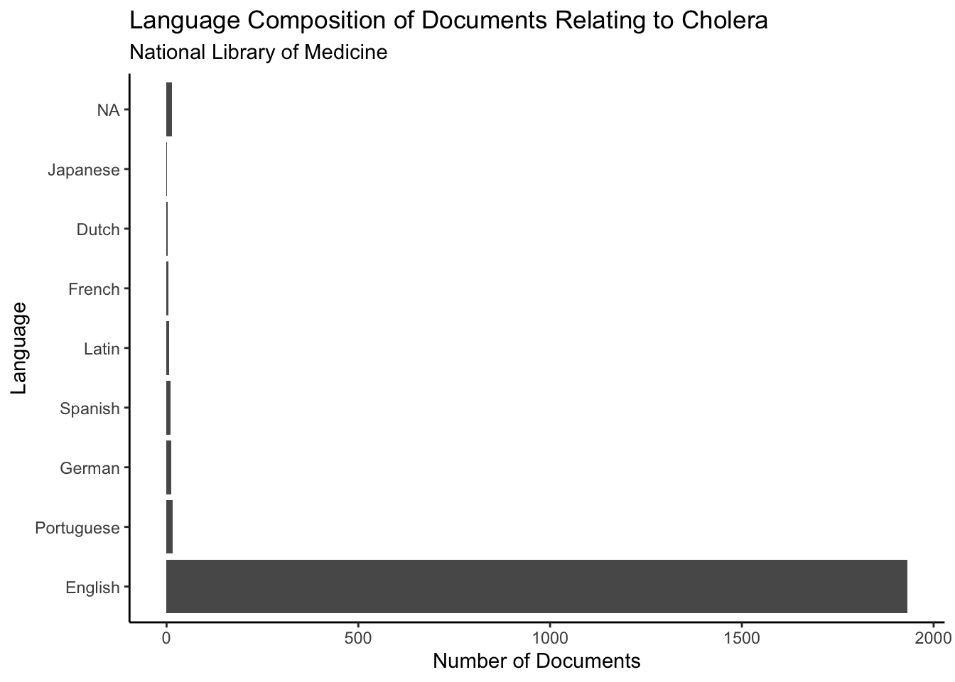
Let’s see if there is correlation between language and publication date. To do so, we will produce density plots over time where the color of the line varies by language. Density plots can be thought of as a sort of smoothed histogram. You can read more about them here.
cholera %>%
  mutate(date = as.numeric(date)) %>%
  filter(date > 1750,
         !is.na(language)) %>%
  ggplot(aes(x = date, color = language)) +
  geom_density() +
  theme_classic() +
  labs(x = "Date",
       y = "Density of Publications",
       color = "Language",
       title = "Cholera Documents in NLM Database by Year and Language")
## Warning: Groups with fewer than two data points have been dropped.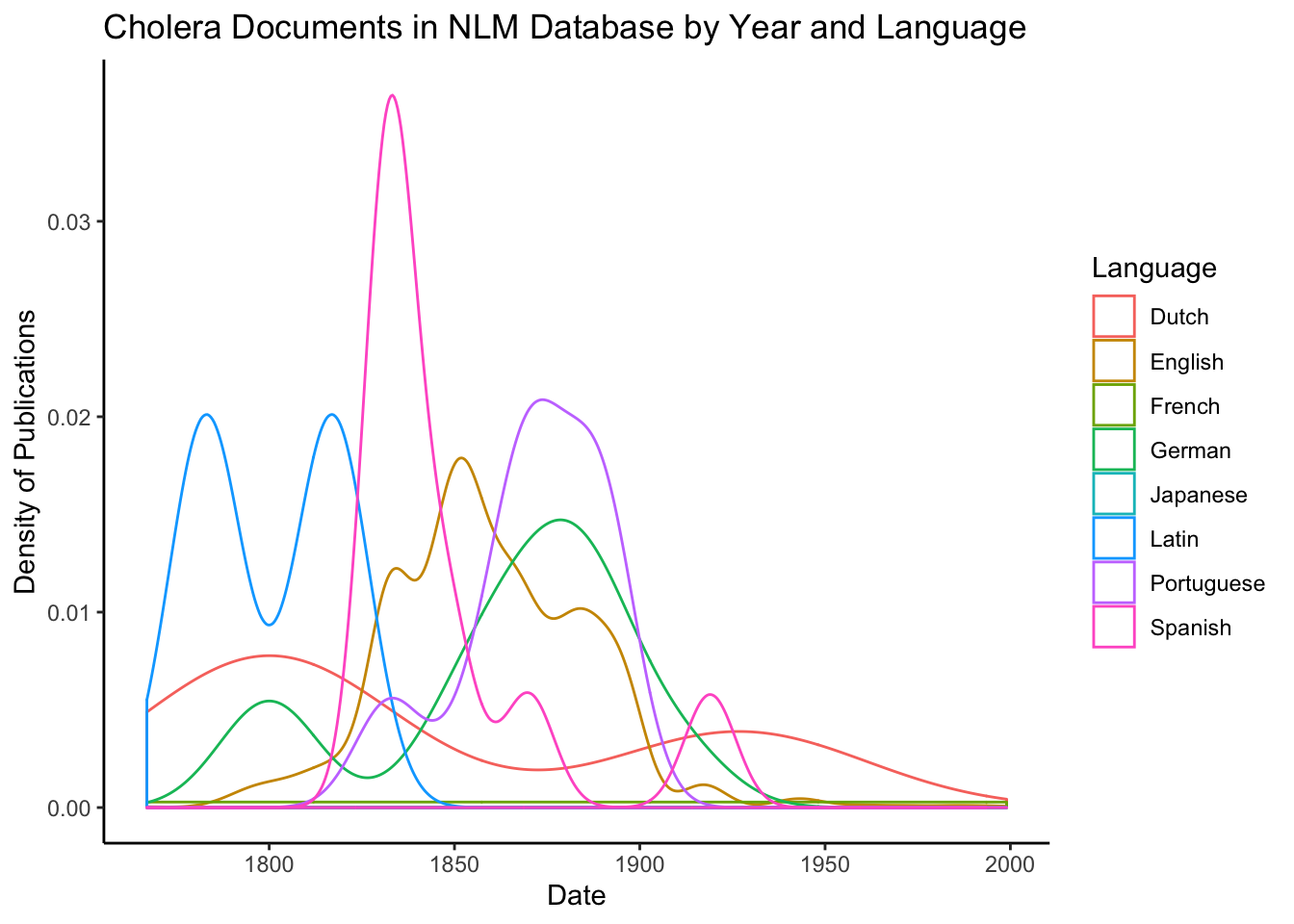
The figure above indicates that there may be some correlation between date of publication and language. It appears that English language publications peaked in 1850 and almost entirely ceased by 1900. In contrast, Portuguese and German publications peaked in the late 1800s, and Spanish publications peaked in the early 1800s. Of course, given the low number of entries that were not in English, this correlation might just be statistical noise. I do not have a comprehensive explanation for these results, but the early peak of Spanish might be related to former Spanish colonies gaining their independence.
Cholera Publications by Geography
Finally, we can look at the geography of publications relating to Cholera. To do so, we will group_by coverage and aggregate with count. This shows how many documents there are for each geographical area. Next, we will use top_n so that only the ten most common geographies are shown. This prevents the chart from being cluttered with fairly irrelevant geographies. As can be seen below, nine out of the ten most frequent geographies in the dataset are located in the USA or the UK. The one exception, India, was a British colony when the majority of the documents in the dataset were written. This demonstrates a bias in the archival policies of the National Library of Medicine, in the publication of documents relating to Cholera, or both.
cholera %>%
  filter(!is.na(coverage)) %>%
  group_by(coverage) %>%
  count() %>%
  ungroup() %>%
  top_n(10) %>%
  ggplot(aes(x = coverage, y = n)) +
  geom_col() +
  theme_classic() +
  coord_flip() +
  labs(title = "Top Ten Cholera Geographies",
       subtitle = "National Library of Medicine",
       x = "Geographical Coverage",
       y = "Number of Documents")
## Selecting by n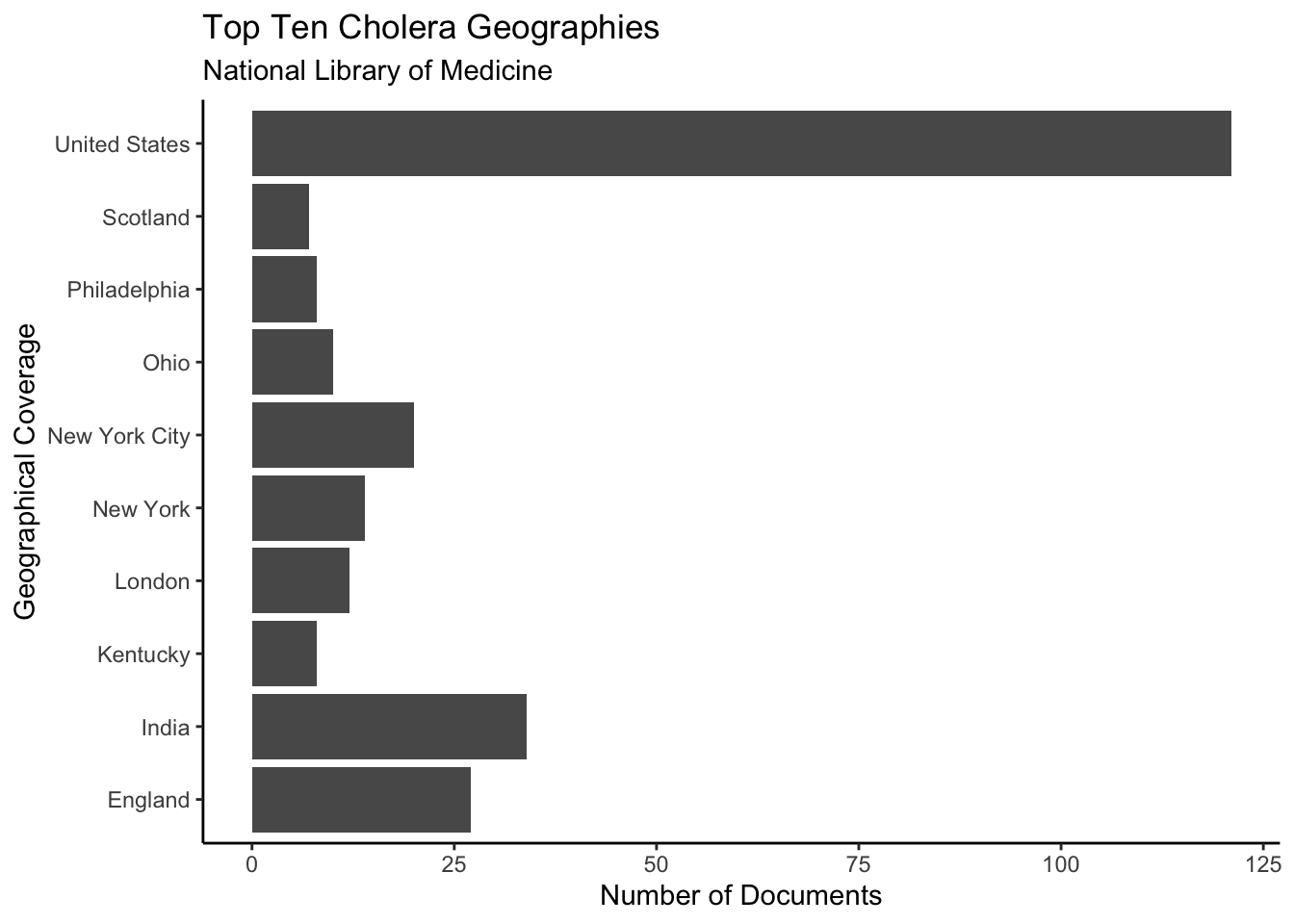
(The code for this section of the blog post is borrowed from the Cholera vignette of tidynlm.)
Conclusion
tidynlm is a convenient API wrapper for accessing the National Library of Medicine document archives. It currently allows an R user to query the NLM database for documents with searchnlm, and then easily visualize the results. After using it to examine Cholera publications, I can conclude that medical research on Cholera seems to have peaked in the late 19th century, and that either research was concentrated in the USA and UK or that the National Library of Medicine does not provide an unbiased sample of medical research (or both).