Machine Learning from Scratch: Classifying Legendary Pokemon with tidymodels
Gabe Preising
So machine learning is all the rage now, huh? I figured as a broke college student who doesn’t know what he’s doing with his life but knows how to code, this would probably be a good thing to learn. I have zero experience with this topic, minimal experience with any math beyond basic statistics, and I never got a chance to take machine learning classes in college due to scheduling conflicts. But now that I can’t leave my apartment since we’re in a pandemic, what better time to learn?
The goal of this project is for me to a) learn how machine learning and predictive modeling works and b) implement some of the features of the recently released tidymodels package from Max Kuhn’s group at RStudio. I was inspired to take on this project when I saw this DataCamp tutorial on predicting whether or not certain Pokemon are legendary Pokemon. I loved Pokemon growing up, so this project seemed perfect for me. But again, as a broke college student, there’s no way in hell I’m paying 34 dollars a month to learn something I could teach myself for free. Therefore, my ultimate goal is to reverse-engineer that DataCamp tutorial using tidymodels to make a classifier for legendary Pokemon, and from that model, extract the variables that contribute to their “legendary-ness”.
For context, certain Pokemon are considered legendary. There are anywhere from 5 to 17 legendary Pokemon per generation, and these Pokemon are typically very powerful and make great additions to a player’s team. Some of these can be obtained by normal gameplay and are involved with the story line, whereas others are only attainable from special events. As a result, there typically only exists one of each legendary Pokemon in the games, so a player only has one chance to capture it for their team, unlike other common Pokemon.
The Pokemon dataset downloaded from Kaggle was scraped from Serebii, a Pokemon database. This dataset contains a number of variables (n = 41) related to the specific stats and general classifications for a given Pokemon, making it useful for machine learning. To start learning machine learning, I went through the series of workshop slides from rstudio::conf(2020). Thanks to Kelly McConville’s MATH 241 course at Reed College, I met all the prerequisites for learning tidymodels according to Kuhn (nice!). The first step in making a classifier for legendary Pokemon would be loading the necessary libraries. Max Kuhn also supplied two helper functions that I’ll come back to later, but they’ll be added to this chunk as well.
library(tidyverse)
library(tidymodels)


fit_split <- function(formula, model, split, ...) {
  wf <- workflows::add_model(workflows::add_formula(workflows::workflow(), formula, blueprint = hardhat::default_formula_blueprint(indicators = FALSE)), model)
  tune::last_fit(wf, split, ...)
}


get_tree_fit <- function(results) {
  results %>%
    pluck(".workflow", 1) %>%
    pull_workflow_fit()
}
The next step is wrangling the data, as there were a couple issues that needed to be addressed before the data was usable. For starters, I did some crude data wrangling. I noticed that 20 Pokemon had incorrectly scraped data for height, weight, and secondary type. After looking on the Serebii pages for each of these Pokemon, I realized that these Pokemon had alternate forms with alternate values for these variables, and that whatever data scraping script was used couldn’t parse these alternate values. Since there were only 20 Pokemon with this issue, I just manually edited the dataset to fix the incorrect values (questionable move; maybe reconsider this in your own workflows). Next, since many tidymodels packages can only work with factor and numeric variables, I converted any character variables to factors using mutate. The variable capture_rate should be numeric, but it was a factor, so I coerced it into a numeric variable. Finally, I had to remove NA values from the dataset. The main source of NA variables was in the percentage_male, due to the fact that many Pokemon do not have a sex; therefore, I added the factor variable is_sexless with levels “yes” and “no”. I then converted all NA values in percentage_male to 0. Finally, I converted any NA values in type2 to “None”. I created a new data frame clean_pokemon which excluded extraneous information (japanese_name, classfication, and base_total). At this point, clean_pokemon was ready for downstream analyses.
pokemon <- read_csv("pokemon.csv")

clean_pokemon <- pokemon %>%
  mutate(is_legendary = as.factor(case_when(is_legendary == 1 ~ "yes",
                                            is_legendary == 0 ~ "no")),
         generation = as.factor(generation),
         type2 = case_when(is.na(type2) == TRUE ~ "None",
                           is.na(type2) == FALSE ~ type2),
         is_sexless = case_when(is.na(percentage_male) == TRUE ~ "yes",
                                   is.na(percentage_male) == FALSE ~ "no"),
         percentage_male = case_when(is.na(percentage_male) == TRUE ~ 0,
                                     is.na(percentage_male) == FALSE ~ percentage_male),
         abilities = as.factor(abilities),
         capture_rate = as.numeric(capture_rate),
         name = as.factor(name),
         type1 = as.factor(type1),
         type2 = as.factor(type2),
         is_sexless = as.factor(is_sexless)
         ) %>%
  select(-c(japanese_name, classfication, base_total)) %>%
  arrange(pokedex_number)

#see how many legendary pokemon there are
clean_pokemon %>%
  select(is_legendary) %>%
  group_by(is_legendary) %>%
  summarise(n())
## # A tibble: 2 x 2
## is_legendary `n()`
## <fct> <int>
## 1 no 731
## 2 yes 70Now for the machine learning bit. According to Max Kuhn’s presentation, the goal of machine learning is to “construct models that generate accurate predictions for future, yet-to-be seen data”. There are several types of machine learning, but this project will focus on supervised machine learning: machine learning where there is a ground truth to compare predictions against. A disclaimer: I am barely scratching the surface of machine learning, so please don’t think of this as an exemplary workflow; think of it as a minimum working product. That being said, the first step in preparing a supervised machine learning model is to partition the dataset into a training set and a testing set. The training set will be used to actually construct the model, whereas the testing set will be used to test the accuracy of the model once it is constructed. To do this, I use the function initial_split() from the package rsample. To maintain the population distribution of legendary Pokemon, I performed stratified sampling on the is_legendary variable. I also performed an 80/20 split for partitioning the data into training and testing, respectively.
set.seed(100)
pkmn_split <- initial_split(clean_pokemon, strata = is_legendary, prop = 4/5)
There are also many types of classification models, but to try and reproduce the DataCamp tutorial, I opted for a random forest model since that’s what they used. To understand a random forest model, one must understand what a decision tree is. A decision tree is a unidirectional data structure used for classifying outcomes in the context of machine learning. The decision tree starts at the root and based on the outcomes for a given variable, will split into multiple nodes. This process will repeat until nodes can no longer be split, at which point these final nodes are called “leaves” and will determine the class of the outcome. A random forest generates multiple decision trees to make a more refined model; the use of many machine learning models like this is referred to as an ensemble. The decision trees in a random forest are generated from bootstrapping (uniform sampling with replacement) the training set. The outcomes of these trees are then aggregated into an average decision tree, which is then used for the final fitted model. This process as a whole is known as “bagging” (bootstrap-aggregating).
I used every variable as a predictor for my random forest of 100 trees. I set the “engine” of the model to “ranger”, which just means I’m constructing the model using the package ranger. I also specified that I wanted the model to compute variable importance for the final model to see what makes legendary Pokemon legendary. I set the mode of the model to classification, since that’s what I’m trying to do. tidymodels is very verbose, which is nice if you’re learning this from scratch.
#specify ML mode
rf_spec <- rand_forest(mtry = .preds(), trees = 100) %>%
  set_engine("ranger", importance = "permutation") %>%
  set_mode("classification")
I then fit my training set to the model using the helper function fit_split() from Max Kuhn’s presentation. This is equivalent to last_tune() from the package tune, but just makes it more explicit. fit_split() takes the split object from rsample and considers both the training set and the testing set, so it will train and test the model in one command. We can now look at the metrics for the model.
#fit training data to model
set.seed(100)
rf_fitted <- fit_split(is_legendary ~ .,
                    model = rf_spec,
                    split = pkmn_split)

rf_fitted %>%
  collect_metrics()
## # A tibble: 2 x 3
## .metric .estimator .estimate
## <chr> <chr> <dbl>
## 1 accuracy binary 0.988
## 2 roc_auc binary 0.999rf_fitted %>%
collect_predictions() %>%
roc_curve(truth = is_legendary,
estimate = .pred_yes) %>%
ggplot(aes(x = 1 - specificity,
y = sensitivity)) +
geom_line(
color = "midnightblue",
size = 1.5
) +
geom_abline(
lty = 2, alpha = 0.5,
color = "gray50",
size = 1.2
) +
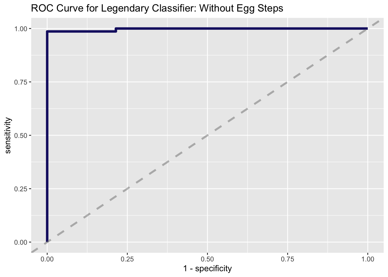
ggtitle("ROC Curve for Legendary Classifier")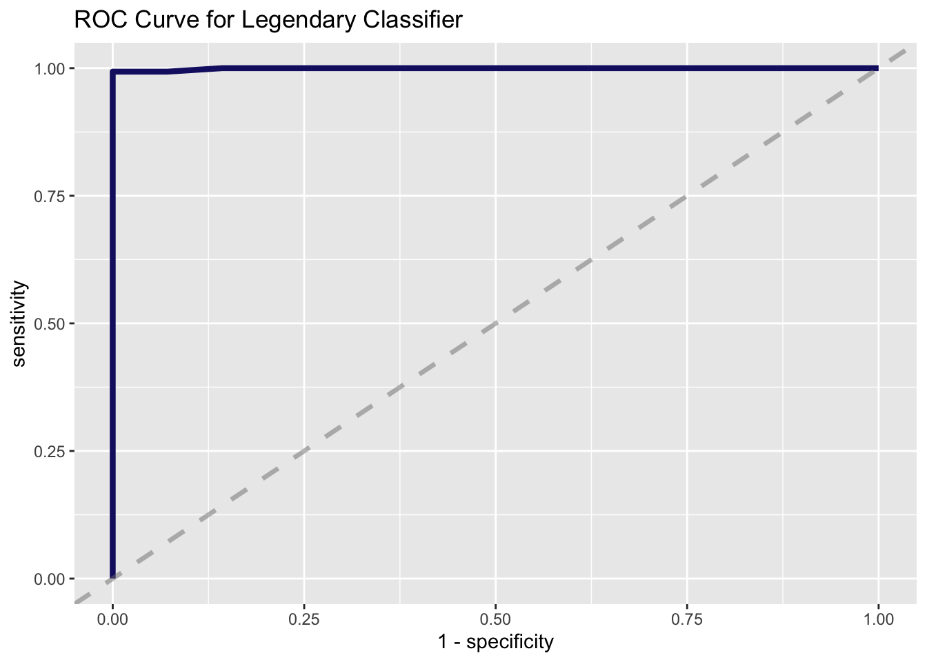
This model has almost 99% accuracy, which is pretty close to perfect. Receiver operator characteristic curves compare the true positive rate (sensitivity) and false positive rate (1 - specificity) of a binary classifier. A perfect receiver operator characteristic curve will have an area-under-the-curve (AUC) value of 1, which this model almost has. A model that randomly guesses would have an AUC value of 0.5, so at least this model isn’t just guessing. Let’s see what variables are driving the strength of this model:
rf_fitted_vip <- get_tree_fit(rf_fitted)
vip::vip(rf_fitted_vip, geom = "col", num_features = 10)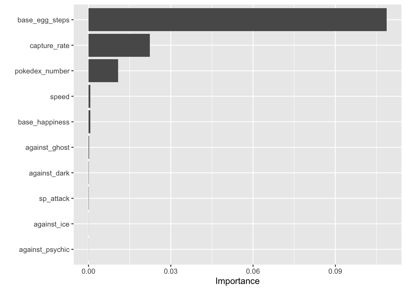
ggplot(clean_pokemon, aes(x = is_legendary, y = base_egg_steps)) +
  geom_boxplot()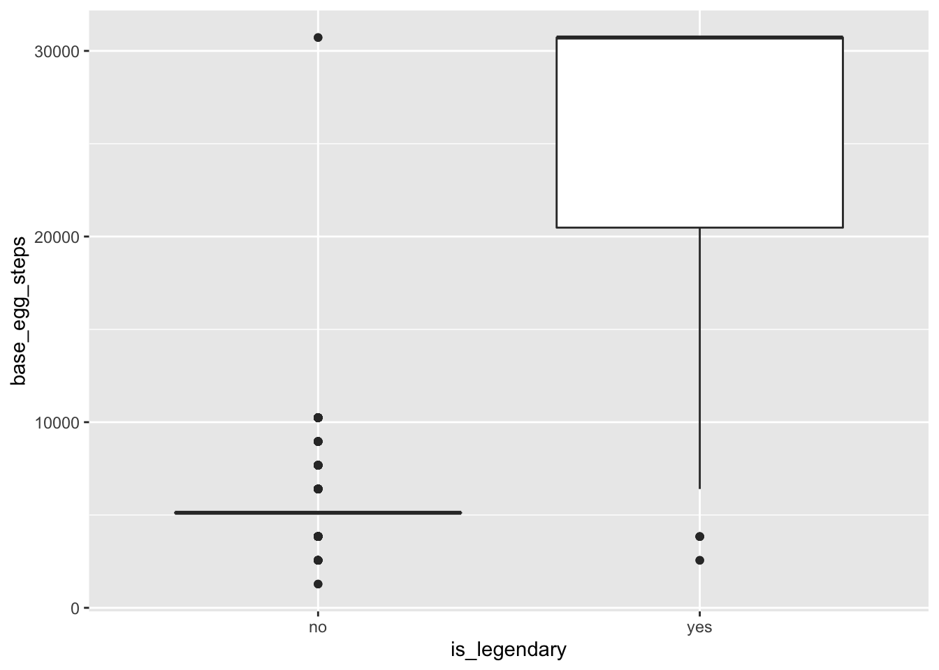
This plot uses the importance values generated from the initial random forest model. Based on the importance ranking, base_egg_steps is clearly driving accurate predictions. In Pokemon, you can hatch eggs to get new Pokemon by walking around in-game with a given egg. After looking at the data, it seems like legendary Pokemon take an egregiously large number of steps to hatch their corresponding eggs. The one caveat is: you can’t get eggs for legendary Pokemon without hacking the game. Therefore, I wanted to get a better set of predictors, so I ran the whole pipeline again, only this time without base_egg_steps as a variable:
## # A tibble: 2 x 3
## .metric .estimator .estimate
## <chr> <chr> <dbl>
## 1 accuracy binary 0.981
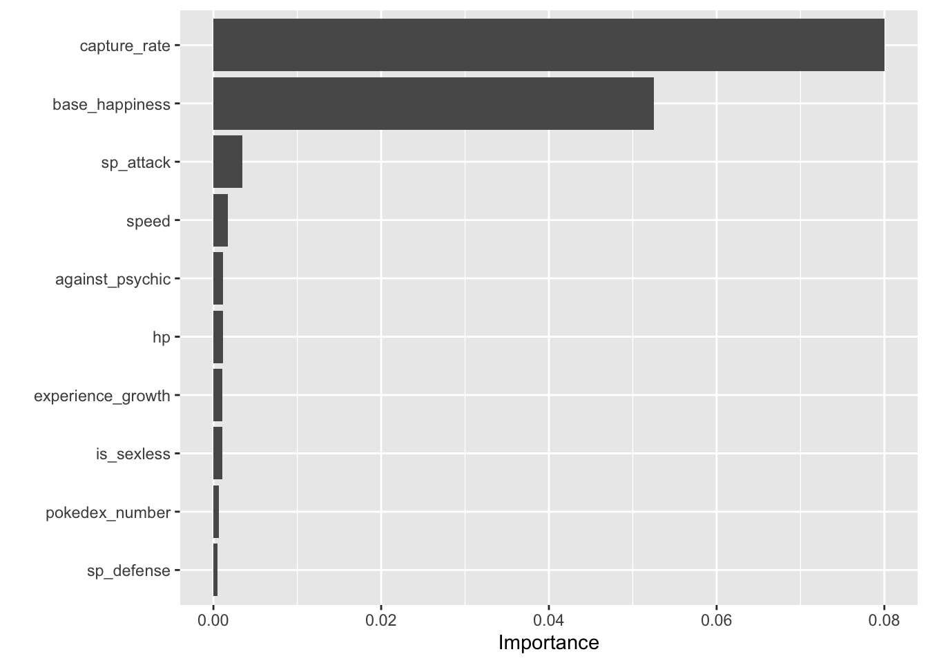
## 2 roc_auc binary 0.997Now, we see a much more diverse set of variables driving accurate predictions. The overall accuracy of the model dropped ever so slightly, which is expected since we removed base_egg_steps.
ggplot(clean_pokemon2, aes(x = is_legendary, y = base_happiness)) +
  geom_violin()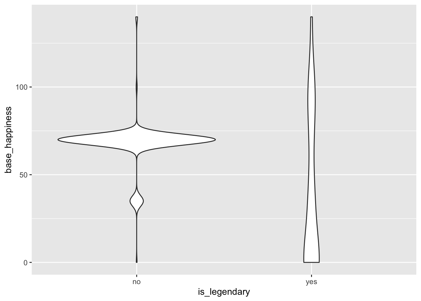
ggplot(clean_pokemon2, aes(x = is_legendary, y = sp_attack)) +
  geom_violin()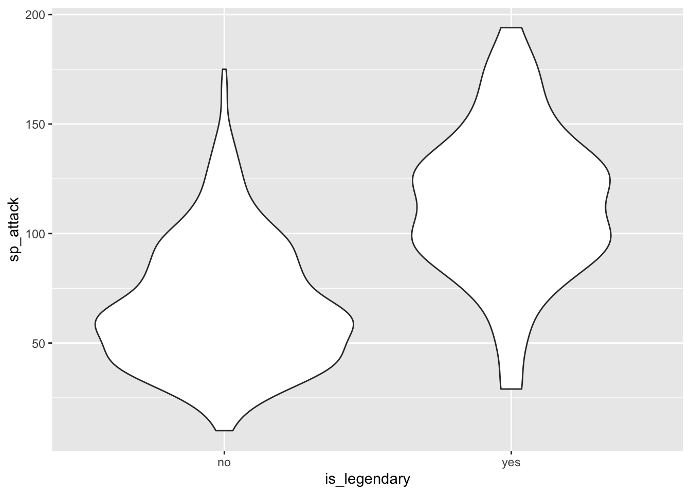
The most important variable in this set is capture_rate, which would make sense since legendary Pokemon are all very difficult to capture. base_happiness is an interesting one, as there is a relatively symmetrical bimodal distribution for legendary Pokemon but more of a contrasting bimodal distribution for non-legendary Pokemon. This may favor extreme happiness values for classifying legendary Pokemon. Finally, legendary Pokemon tend to have a much higher sp_attack value. This variable corresponds to the strength of “special attacks”, or non-physical attacks. This also checks out, since in the games and anime, legendary Pokemon tend to attack with fireballs, lasers, and overall showier moves.
Overall, learning tidymodels was not as hard as I expected.The syntax being similar to that of tidyverse made it really intuitive to learn. While this project just barely got into how machine learning works, it made a very daunting topic very approachable to a beginner. There are a number of aspects I did not touch on in this project due to time constraints, but I look forward to going deeper down this rabbithole. Maybe this skill will end up making me less of a broke college student, and maybe I can pay the damn 34 dollars per month in the future.