Actual vs Predicted Senate Vote compared to Education Levels across U.S. States
David Herrero-Quevedo and Jackson M Luckey
library(tidyverse)
library(tidycensus)
library(tigris) # for loading basemap
library(broom) # for working with the regression
library(knitr) # for kable
library(kableExtra) # so that the tables look less awful.
library(tufte) # so that we can celebrate how amazing Edward Tufte is and how great his books look
Introduction
How much does education levels influence support for Trump? How likely is a senator to vote in favor of Trump considering 2016 election results and the education levels in their state? To answer these question we used FiveThirtyEight’s Tracking Trump In Congress dataset and the U.S. Census Bureau Educational Attainment Survey.
FiveThirtyEight has created three different scores to indicate how senators vote with respect to Trump. The Trump Score represents the percentage of how often a senator votes yes or no and agrees with Trump. The Predicted Score represents how often we would expect a senator agree with Trump based on 2016 election results. The Trump Plus-Minus is derived from the Trump Score minus the Predicted Score. More info on this can be found on FiveThirtyEight here.
Using these scores we will be able to determine the probability of senators voting with the President compared to their constituents’ education levels. We will be analyzing the combined 115th and 116th Congress during the time Donald Trump has been in office.
Data Preparation and Cleaning
We downloaded FiveThirtyEight’s data from their GitHub repo, and loaded it into R with the function read_csv. The data consists of two tables, vote_predictions in which an observation is a representative’s vote, and averages, in which an observation is a representative in a particular session. For this project, we will be using the averages table, as we are interested in the senators’ voting patterns, rather than specific votes.
We then filtered observations to only include Senators from the most recent Congress.
averages <- read_csv("/Users/mcconvil/Desktop/Cumulus/Courses/Spring 2020/math241s20/Projects/MiniProject2/math241S20PostGrp9/averages.csv") %>%
  filter(congress == 0,
         chamber == "senate") %>%
  # drop:
  # chamber because it is "senate" for all observations
  # district because senators are elected on the state level
  # congress because it is "0" for all observations
  select(-chamber, -district, -congress) %>%
  mutate(party = as_factor(party),
         state = as_factor(state))
We used the R Package tidycensus to grab education data from the US Census Bureau. tidycensus helps R users download data from the census without having to learn how to use the census API.
education <- get_acs("State",
                     table = "C15003",
                     output = "wide",
                     survey = "acs1",
                     key = api_key)
After that, we manipulate the columns to create useful, human-readable variables. These are:
- % Less than High School
- % High School
- % GED
- % Some college
- % College
- % Graduate education
We then aggregate these variables into broader categories:
- % highschool or less
- % bachelors or more
With these aggregated variables, we will be able to determine what impact education levels have on a state’s support for Trump and the voting patterns of senators from that state.
education <- education %>%
 rename(population = C15003_001E) %>%
  # create the small education bins
  mutate(education_small_bin_percent_less_than_highschool = (C15003_002E + C15003_003E + C15003_004E + C15003_005E + C15003_006E + C15003_007E + C15003_008E + C15003_009E) / population,
         education_small_bin_percent_highschool = C15003_010E / population,
         education_small_bin_percent_ged = C15003_011E / population,
         education_small_bin_percent_some_college = (C15003_012E + C15003_013E + C15003_014E) / population,
         education_small_bin_percent_college = C15003_015E / population,
         education_small_bin_percent_graduate = (C15003_016E + C15003_017E + C15003_018E) / population) %>%
  # add up the small bins into the bins we'll use
  mutate(education_high_school_or_less = education_small_bin_percent_ged + education_small_bin_percent_highschool + education_small_bin_percent_less_than_highschool,
         education_bachelors_or_more = education_small_bin_percent_college + education_small_bin_percent_graduate) %>%
  # rename the variable to make future merging easier
  rename(state = NAME) %>%
  # drop the variables we no longer need (the raw estimates and margins of error)
  select(GEOID, state, population, starts_with("education"))
In order to draw maps, we will require a base map. A base map is a blank map that data can be mapped onto. We can download one from the tigris package with the following code:
# download state geometry files
base_map <- states(cb = TRUE, class = "sf", progress_bar = FALSE) %>%
  select(geometry, state = STUSPS, NAME)

theme_tufte <- theme(panel.background = element_rect("#fffff8", "#fffff8"),
                     plot.background = element_rect("#fffff8", "#fffff8"))
We then aggregate the voting data by state, use joins to add in a base map and education data, and drop Alaska and Hawaii to simplify map-drawing.
df <- averages %>%
  group_by(state) %>%
  summarize(trump_vote = mean(net_trump_vote),
            predicted_agree = mean(predicted_agree),
            actual_agree = mean(agree_pct)) %>%
  left_join(base_map, by = c("state" = "state")) %>%
  rename(state = NAME, state_code = state) %>%
  left_join(education, by = c("state" = "state")) %>%
  filter(!(state %in% c("Hawaii", "Alaska"))) %>% # exclude Alaska and Hawaii because they don't fit on the map
  select(-GEOID) # we won't need it
## Warning: Column `state` joining factor and character vector, coercing into
## character vectorWhere did Trump do well in 2016?
Now that we’ve cleaned and prepared our data, we’re ready to draw some maps. ggplot2 can draw maps from tigris or tidycensus using geom_sf. Let’s start by drawing a map of Trump’s support in the 2016 election.
ggplot(df, aes(fill = trump_vote, geometry = geometry)) +
  geom_sf() +
  theme_map +
  xlim(-125, -68) +
  ylim(23, 50) +
  scale_fill_distiller(type = "div", palette = "RdBu") +
  labs(fill = "Margin (%)",
       title = "Trump's Share of the 2016 Election Votes Minus Clinton's") +
  theme_tufte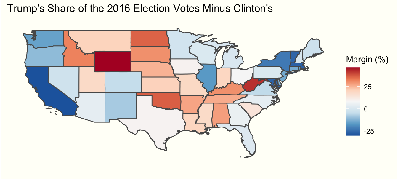
Based off of the map, it is apparent that Trump has significantly more support in the middle of the country than either coast. Wyoming and California stand out as the most polarized.
Does having a bachelor’s influence support for Trump?
Now let’s test whether or not having a bachelor’s degree or more influences support for Trump. We can do this by running a regression, which tests whether or not an explanatory variable affects an outcome. We can then grab the results of the regression with the function tidy from the broom package, which helps R users work with regressions. As shown by the table below, states where a higher percentage of the population has a bachelor’s degree or more cast relatively fewer votes for Donald Trump in 2016.
tidy(lm(trump_vote ~ education_bachelors_or_more, df)) %>%
  # drop the intercept term, as we are only interested in the direction of the effect
  filter(term != "(Intercept)") %>%
  select(term, estimate) %>%
  # make the explanatory variable name nice and human readable
  mutate(term = if_else(term == "education_bachelors_or_more",
                        "Having a bachelor's degree or more",
                        term)) %>%
  kable(col.names = c("Explanatory Variable", "Effect on Voting for Trump")) %>%
kable_styling(position = "float_left")| Explanatory Variable | Effect on Voting for Trump |
|---|---|
| Having a bachelor’s degree or more | -269.9827 |
Now let’s look at which states bucked this trend. Regressions produce residuals, meaning the difference between what the explanatory variable predicts and what actually happened. We can extract the residuals using the base R function resid and attach them to the dataframe using a mutate call.
# confirmed that this works: https://stackoverflow.com/questions/20506984/are-residuals-in-linear-regression-following-same-order-of-original-data-frame-r
df <- df %>%
  mutate(college_or_more_support_residual = resid(lm(trump_vote ~ education_bachelors_or_more, df)))
Now that we’ve made the residuals a column in the dataframe, we can draw a map of them. This allows us to see which states voted for Trump more or less than their education levels would predict.
ggplot(df, aes(fill = college_or_more_support_residual, geometry = geometry)) +
  geom_sf() +
  theme_map +
  xlim(-125, -68) +
  ylim(23, 50) +
  scale_fill_distiller(type = "div", palette = "RdBu") +
  labs(title = "Which states voted for Trump more than their education levels predicted?",
       fill = "Positive is More") +
  theme_tufte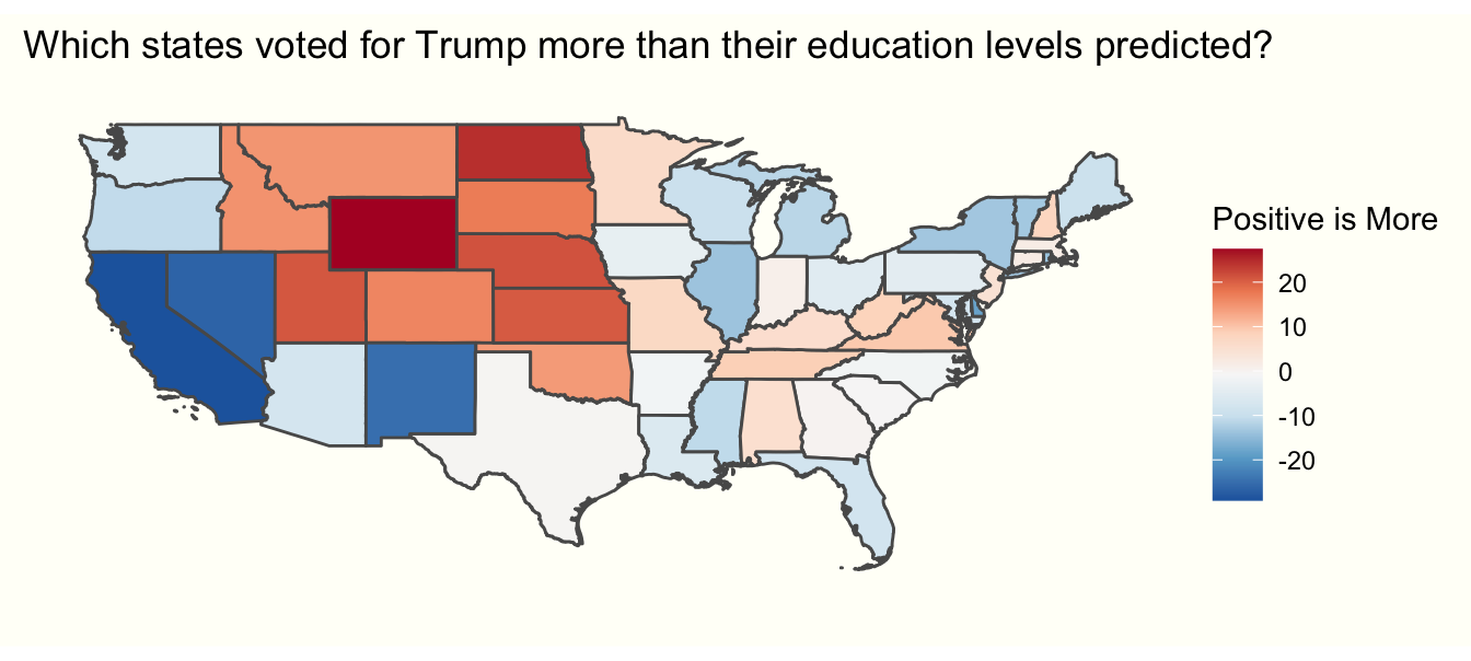
From the above map, we can see that certain states, such as Wyoming, voted for Trump at much higher levels than expected, whereas Trump underperformed in Nevada, California, and New Mexico relative to those states’ education levels. Let’s examine these observations (and Ohio as a control) to see what is going on. To do so, we’ll subset the data using a filter.
df %>%
  filter(state %in% c("Wyoming", "Ohio", "California", "Nevada", "New Mexico")) %>%
  mutate(education_bachelors_or_more = education_bachelors_or_more * 100) %>%
  select(state, trump_vote, education_bachelors_or_more, college_or_more_support_residual) %>%
  kable(col.names = c("State", "Trump Vote Share", "Bachelors or More %", "Vote Relative to Education")) %>%
kable_styling(position = "float_left")| State | Trump Vote Share | Bachelors or More % | Vote Relative to Education |
|---|---|---|---|
| Ohio | 8.129574 | 28.97222 | -5.009677 |
| Wyoming | 46.295276 | 26.85661 | 27.444249 |
| Nevada | -2.417128 | 24.88984 | -26.578082 |
| California | -30.109293 | 34.20047 | -29.133167 |
| New Mexico | -8.213268 | 27.65388 | -24.911794 |
Looking at the table, it appears that Wyoming is an outlier simply because it voted overwhelmingly for Trump. This is likely due to its extremely rural, conservative nature. The opposite is true of California. In contrast, both Nevada and New Mexico simply voted less for Trump than their education levels would predict.
Do senators vote differently depending on their constituents’ education levels?
ggplot(df, aes(fill = actual_agree, geometry = geometry)) +
  geom_sf() +
  theme_map +
  xlim(-125, -68) +
  ylim(23, 50) +
  scale_fill_distiller(type = "div", palette = "RdBu") +
  labs(title = "Which senators vote with Trump?",
       fill = "% of the Time") +
  theme_tufte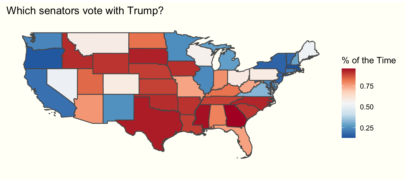
Now let’s examine whether or not a senator’s constituents’ education level affects their voting pattern. First, we’ll run a regression to see how it affects voting patterns. As shown by the table below, senators with a more highly educated constituency vote with Trump less often.
tidy(lm(actual_agree ~ education_bachelors_or_more, df)) %>%
  filter(term != "(Intercept)") %>%
  select(term, estimate) %>%
  mutate(term = if_else(term == "education_bachelors_or_more",
                        "Having a bachelor's degree or more",
                        term)) %>%
  kable(col.names = c("Explanatory Variable", "Effect on Senator Agreeing with Trump")) %>%
kable_styling(position = "float_left")| Explanatory Variable | Effect on Senator Agreeing with Trump |
|---|---|
| Having a bachelor’s degree or more | -3.758465 |
After adjusting for education, the map looks like:
df <- df %>%
  mutate(college_or_more_senator_residual = resid(lm(actual_agree ~ education_bachelors_or_more, df)))
ggplot(df, aes(fill = college_or_more_senator_residual, geometry = geometry)) +
  geom_sf() +
  theme_map +
  xlim(-125, -68) +
  ylim(23, 50) +
  scale_fill_distiller(type = "div", palette = "RdBu") +
  labs(title = "Educated-adjusted Senator Voting Patterns",
       fill = "Voting with Trump") +
  theme_tufte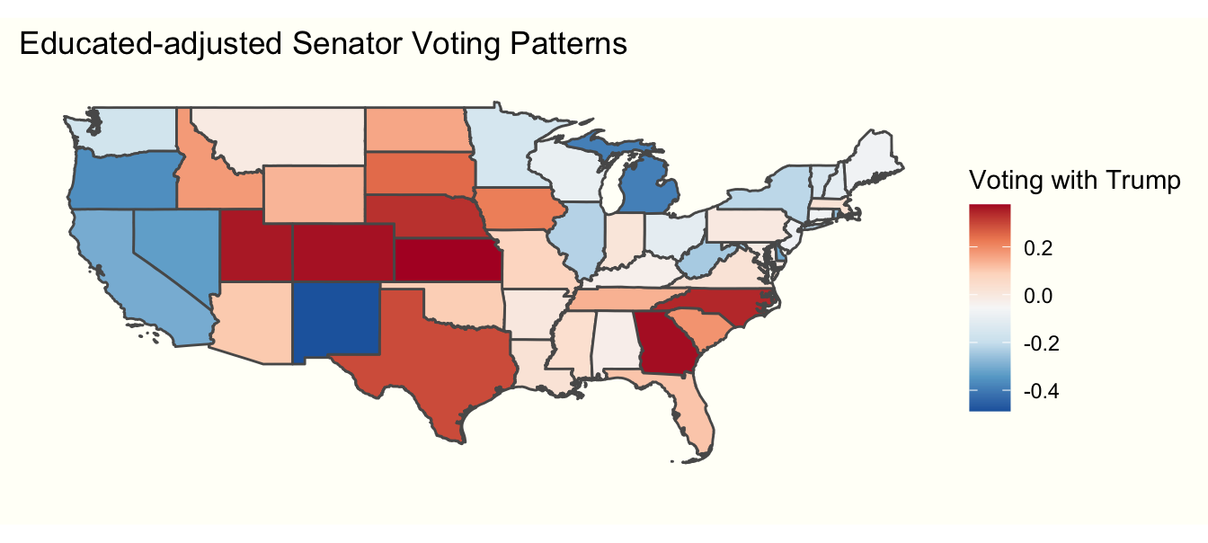
After adjusting for education, there are some major changes in senators’ voting patterns. The partisan lean of most of the south is significantly reduced, suggesting that a lack of education among their constituents explains why southern senators vote with Trump. Georgia and North Carolina buck this trend. Anecdotally, in North Carolina this is likely due to the highly educated members of the population being concentrated in the Raleigh-Durham-Chapel Hill metro area. Interestingly, senators from Utah, Colorado, Kansas, and Nebraska all vote with Trump much more often than education would predict. we suspect this also has to do with geographic clustering of the highly educated members of their populations. Finally, senators from New Mexico vote for Trump far less than education would predict.
Conclusion
While education did a fairly good job of explaining voting for Trump at both the constituent and senator level in some states, it did not in others. Geographic distribution of the highly educated part of the population explains this disparity in a few states, such as North Carolina. In the remaining states, other factors must be at play. Scholarly work on the other predictors of support for Donald Trump can be read here, here, or here.